Viking 2-D — end-to-end example¶
Reproduces the Mobil AVO Viking Graben (line 12) FWI + RTM result with the sweep-tasks CLI, starting from the public S3 download and ending at a filtered RTM image. The walkthrough below assumes you are running locally on a single workstation with one GPU — no SLURM, no cluster filesystem layout. A short § Running on a cluster (optional) appendix at the end shows the ibex-style sbatch entry points if you want them.
download → build-index → build-plan ┐
                                     ├─ wavelet (legacy) ┐
                                     └─ initial model (legacy) ┤
                                                                └─ FWI → RTM → filter-image
The end-to-end pipeline matches the legacy fwi_workflow-dev
reference number-for-number. Indexing, plan-building, wavelet
estimation (rank-1 average + SIREN/sweep refinement), FWI, RTM, and
the depth-tapered post-filter all live inside sweep-tasks; only the
initial velocity model builder is still served by a legacy
script (TODO: port, see § Roadmap).
Visual tour — what each step produces¶
Every sweep-tasks command in the pipeline writes at least one
preview PNG by default (use --no-qc-png or --no-plot to disable).
Only the steps verified end-to-end against the Viking dataset are
shown below; the remaining steps (3b, 3d, 6, 7) will be added once a
clean reference run is captured.
| Step | One-line product | Visual |
|---|---|---|
1 build-index |
SEG-Y per-trace catalog (3-panel geometry QC) | 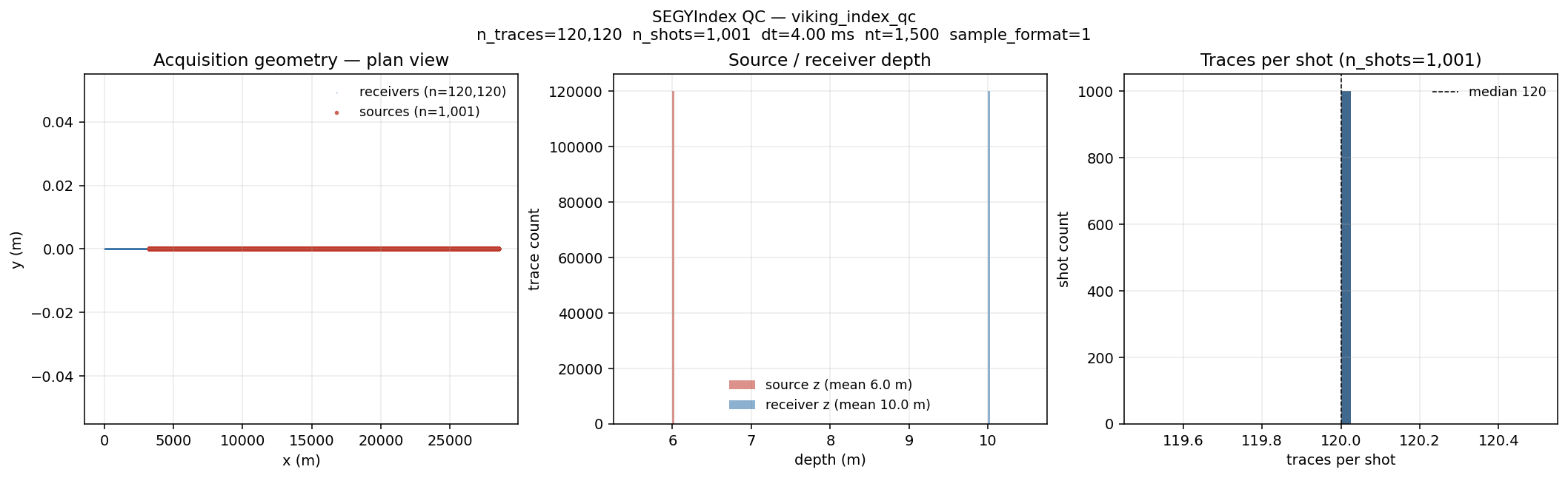 |
2 build-plan |
Filtered + grouped plan (3-panel filter QC) | 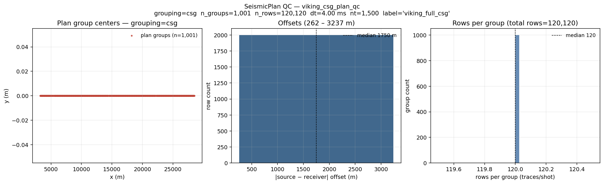 |
3a analyze-wavelet |
Robust direct-wave average across all shots | 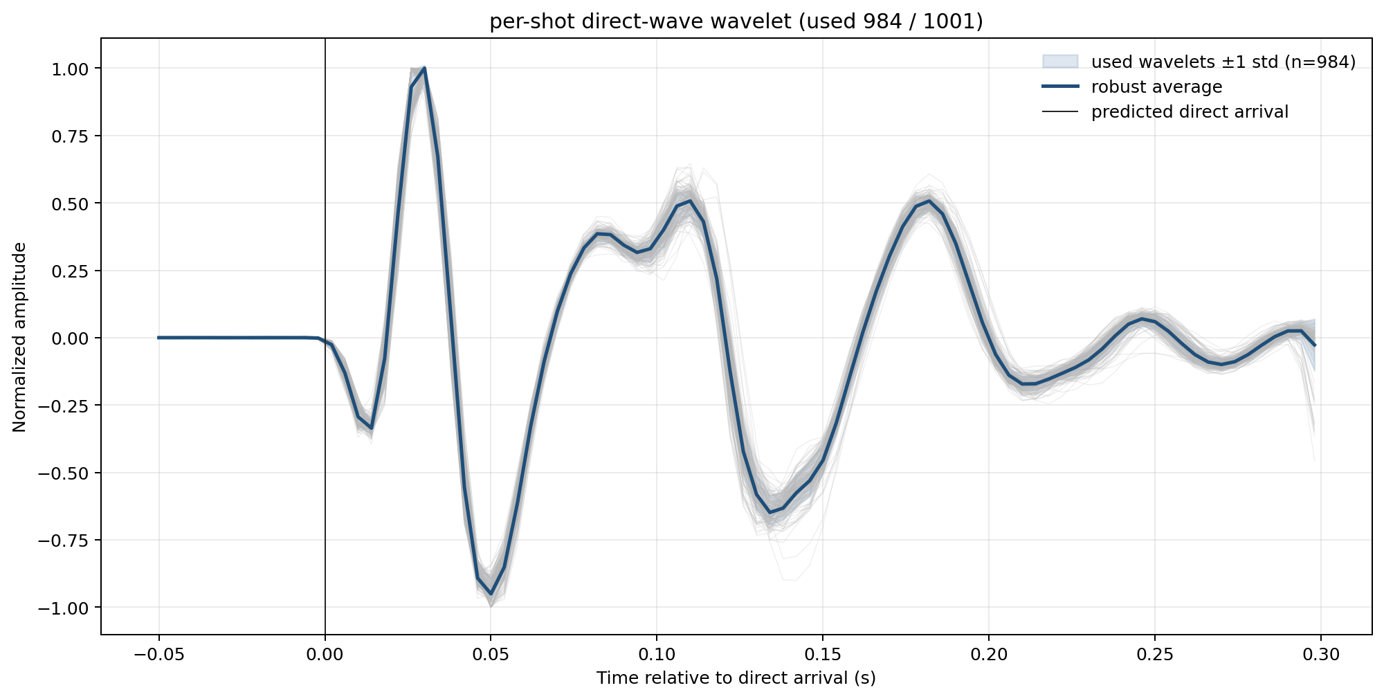 |
3c convert-farfield |
Far-field signature (QC reference) | 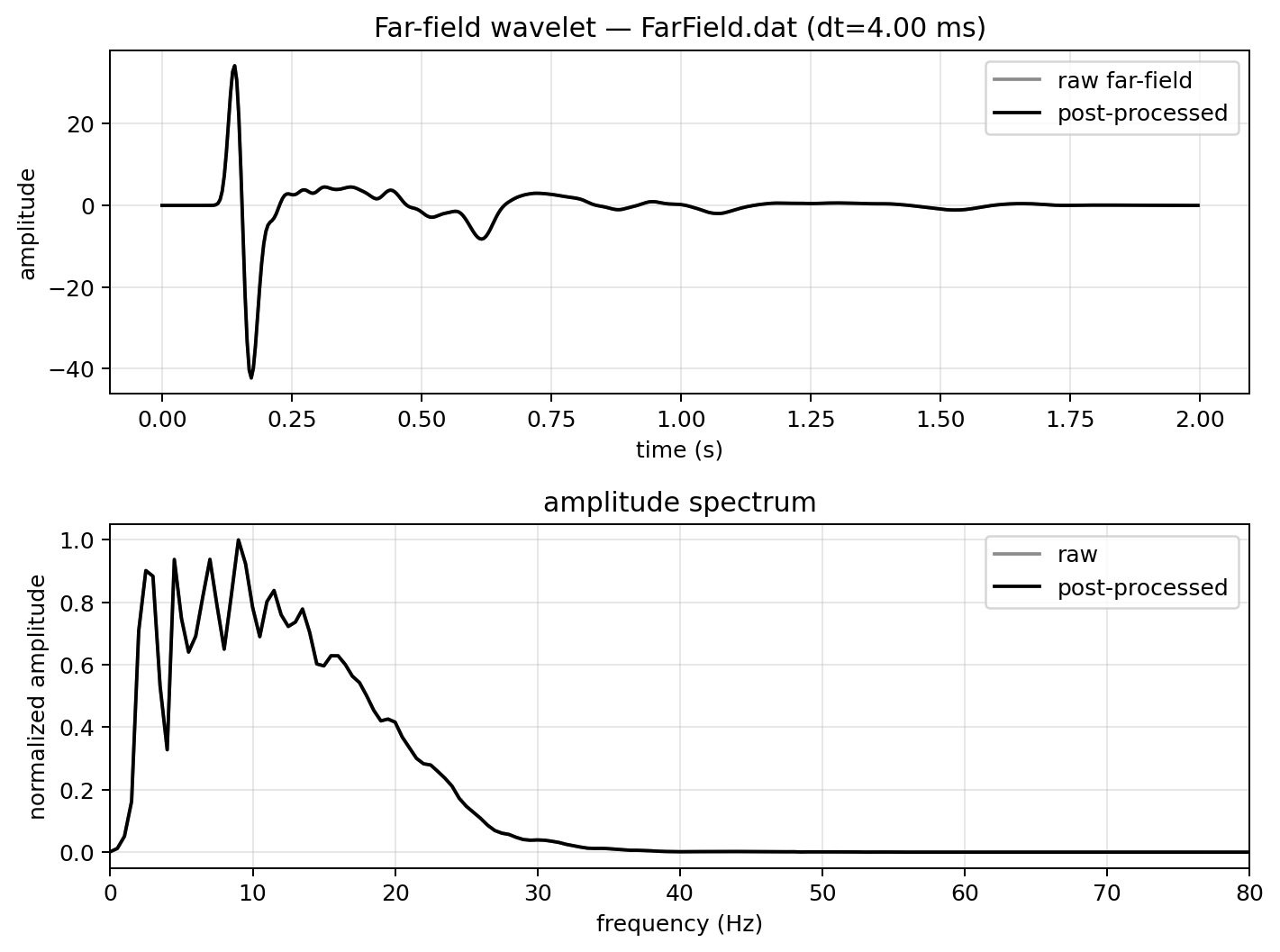 |
| 5 freqsel FWI | Inverted vp from a 1-D cold start, 10 min | 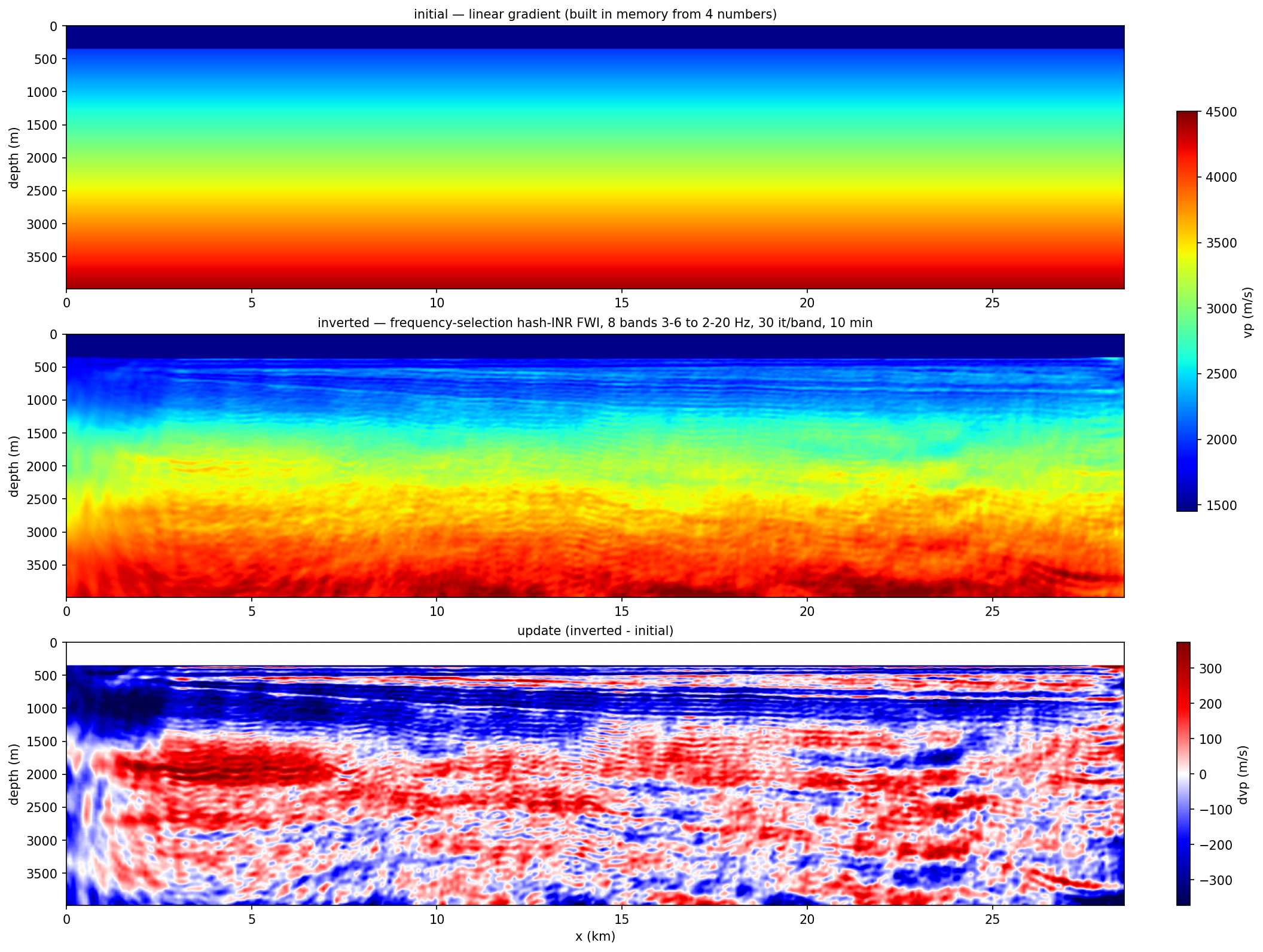 |
Prerequisites¶
- Sweep installed. From a checkout of this repo:
pip install -e sweep            # propagator
pip install -e sweep-io         # SEG-Y readers, SeismicPlan
pip install -e sweep-tasks      # the CLI entry points used below
- One CUDA-capable GPU. Anything with ≥ 16 GB works for Viking at the 12.5 m grid (24 GB recommended for the full 6-stage ladder). Sanity check:
- Working directory. Pick one writable folder for the whole
pipeline; the doc uses
$VIKING_HOMEeverywhere. Around 5 GB free is plenty (SEG-Y 750 MB + outputs ~3 GB).
$VIKING_HOME/rawwill hold the downloaded SEG-Y + far-field.$VIKING_HOME/runwill hold the index, the plan, FWI / RTM outputs.
That's all the environment setup. No SWEEP_*_ROOT / PROJECT_DATA_ROOT
exports are needed for local single-GPU runs — those variables only
matter for the cluster sbatch templates discussed at the bottom of
this file.
One file drives every step — sweep-tasks init viking¶
Every command in Steps 1–3d below accepts either a forest of CLI
flags or --config viking.yaml (one YAML, sections per step).
This is the recommended path — no 30-flag invocations to remember.
Generate the starter config with sweep-tasks init:
sweep-tasks init -o $VIKING_HOME/viking.yaml
# wrote 'viking' template -> /home/you/viking/viking.yaml
# next: edit the paths inside (especially $VIKING_HOME / $HOME), then run:
#        sweep-tasks build-index --config /home/you/viking/viking.yaml
(sweep-tasks init --list shows what's bundled. Three templates ship
today: viking (wavelet pipeline, default), fwi (FWI task YAML
for sweep-tasks run), rtm (RTM task YAML). Run without -o to
dump to stdout and pipe / edit directly.)
The generated YAML has one section per subcommand (build_index:,
build_plan:, analyze_wavelet:, estimate_wavelet:,
convert_farfield:, plot_wavelet_steps:) plus a common: block
for shared defaults. All paths inside use $VIKING_HOME so
once that env var is set the file is usable as-is. Open the file
and adjust any value you want different from the canonical Viking
defaults; saving / re-running is enough — no re-init needed.
CLI flags override YAML, so you can adjust one knob at a time without editing the file:
The step-by-step sections below show the --config form as the
primary command and list the full CLI alternative when relevant.
Step 0 — Download the public dataset¶
The data lives in the SEG open-data S3 bucket:
cd $VIKING_HOME/raw

BASE=https://s3.amazonaws.com/open.source.geoscience/open_data/Mobil_Avo_Viking_Graben_Line_12

# Pre-stack SEG-Y (750 MB) — the only file FWI / RTM strictly need.
curl -fL -O ${BASE}/seismic.segy

# Far-field source signature (ASCII, one sample per line; dt = 4 ms).
# NOTE the capital F in FarField — the bucket is case-sensitive and
# `Farfield.dat` returns HTTP 403.
curl -fL -O ${BASE}/FarField.dat

# Optional auxiliary material.
curl -fL -O ${BASE}/mobil_wellogs.tar.gz           # well logs (LIS)
curl -fL -O ${BASE}/Mobil_migration_well_logs.pdf  # wellog plots
curl -fL -O ${BASE}/284E_frontmatter.pdf           # SEG Open Pub No. 4 front matter
curl -fL -O ${BASE}/README.txt
curl -fL -O ${BASE}/sufirst.job
curl -fL -O ${BASE}/FarField.jpg
Sanity-check the bundle:
That byte count is not approximate — it is exactly what the headers imply, so it doubles as an integrity check:
3600 + 120120 x (240 + 1500 x 4) = 749,552,400
^      ^         ^     ^
|      |         |     samples x 4 bytes (IBM float)
|      |         trace header
|      trace count
textual + binary file header
The textual header is a blank SEG-Y template — no client, line or crew filled in — so every acquisition fact below comes from the binary and trace headers, not from the reel stationery.
What's in seismic.segy¶
| Field | Value |
|---|---|
| Trace count | 120,120 (1001 shots × 120 channels) |
| Samples / trace | 1500 |
| Sample interval | 4 ms |
| Record length | 6.0 s |
| Sample format | 1 (IBM 32-bit float) |
| FFID range | 3 to 1003 |
| Shot interval | 25 m |
| Group interval | 25 m |
| Offset range | -262 m (near) to -3,237 m (far) |
| Source x | 3,237 to 28,512 m |
| Receiver x | 0 to 28,250 m |
sy = gy = 0 for every trace — the line is genuinely 2-D in x. SEG-Y
coordinate scalar = 1 (so sx, sy, gx, gy are already metres) and
coord-units = 3 (m). Source / receiver depth bytes are zero, so
Step 1 below injects the canonical Viking acquisition constants:
airgun array at 6 m, streamer at 10 m.
Step 1 — sweep-tasks build-index¶
Scans every SEG-Y trace header in parallel and writes a tiny per-trace catalog. Run once; the same index serves every plan you build later.
Or, equivalently, all-CLI:
sweep-tasks build-index \
    --segy-root  $VIKING_HOME/raw \
    --glob       'seismic.segy' \
    --out        $VIKING_HOME/run/viking_index.npz \
    --num-workers 8 \
    --source-depth-m   6.0 --receiver-depth-m 10.0 \
    --progress
--num-workers 8 finishes Viking in ~10 s on a laptop CPU; bump it
to whatever your machine has. (The -n N MPI shortcut covered in
docs/cli_workflow.md is for much larger
3-D surveys — Viking does not need it.)
Console output (measured on Viking)
[build-index] scanning 1 SEG-Y files under /…/viking/raw (glob='seismic.segy'; threads=8)
  scanned seismic.segy  (file_id=0, traces=120120)
[build-index] scan complete: 120,120 traces across 1 files, dt=0.004s nt=1500, wall=0.5s
[build-index] wrote /…/viking_index.npz (0.3 MB)
[build-index] QC PNG -> /…/viking_index_qc.png
Wall time end-to-end (process startup + scan + npz + PNG): 14 s measured here (8.6 s of that is the scan itself, 8 threads).
Outputs
$VIKING_HOME/run/viking_index.npz(~300 KB) — per-tracefile_id,byte_offset,ffid,sx/sy/sz,gx/gy/gz.source_depth_mandreceiver_depth_marrays are constant at 6 m / 10 m (overrides).viking_index_qc.png(~100 KB) — 3-panel acquisition geometry preview (pass--no-qc-pngto skip).
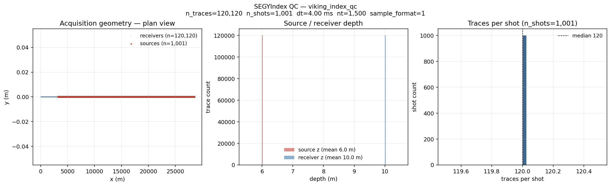
The QC PNG (see Visual tour above) is a 3-panel preview: plan-view
(sources red, receivers blue — Viking is a 2-D line so both
collapse to single tracks along x); source & receiver depth
histograms (sharp peaks at 6 m / 10 m — the constants we injected
via --source-depth-m / --receiver-depth-m); per-shot trace-count
histogram (perfectly flat 120 traces × 1001 shots).
Verify programmatically with:
>>> from sweep_io.segy_index import SEGYIndex
>>> idx = SEGYIndex.load("$VIKING_HOME/run/viking_index.npz")
>>> idx.n_traces, idx.n_shots, idx.dt_s, idx.n_samples
(120120, 1001, 0.004, 1500)
>>> idx.sx_m.min(), idx.sx_m.max()      # positions are sx_m / rx_m, in metres
(3237.0, 28512.0)
Measured on this index, every row of the acquisition table above checks out:
1001 shots of exactly 120 traces, 25 m shot and group interval, |offset|
262-3237 m, sy = ry = 0, and sz / rz constant at the 6 m / 10 m injected
by the flags.
Step 2 — sweep-tasks build-plan¶
Filters + groups the index into a seismic_plan_v1 npz that declares
exactly which trace bytes FWI will read. Plans are cheap to rebuild
— iterate freely on shot subsets, offset windows, sub-sampling, etc.
Full CSG plan (all 1001 shots × 120 receivers)¶
Or all-CLI:
sweep-tasks build-plan \
    --index    $VIKING_HOME/run/viking_index.npz \
    --grouping csg \
    --out      $VIKING_HOME/run/viking_csg_plan.npz \
    --label    "viking_full_csg"
3 km offset cap (for the RTM in Step 6)¶
sweep-tasks build-plan \
    --index         $VIKING_HOME/run/viking_index.npz \
    --grouping      csg \
    --offset-max-m  3000 \
    --out           $VIKING_HOME/run/viking_csg_3km.npz \
    --label         "viking_csg_offset_le_3000m"
Measured here (5.2 s and 4.7 s respectively, index load included):
| plan | groups | rows | |offset| | rows / group |
|---|---|---|---|---|
| full CSG | 1001 | 120,120 | 262 – 3237 m | 120 |
| 3 km cap | 1001 | 110,110 | 262 – 2987 m | 110 |
The cap drops 10,010 rows — 8.3 % of the survey, ten channels off the tail of every shot — and empties no group, which is what you want a filter to do.
Each build-plan invocation also writes <out>_qc.png next to the
npz (pass --no-qc-png to skip). The PNG shows what survived your
filters in three panels: group-center scatter (with dropped
groups underlaid in gray when an --index is supplied), per-row
offset histogram, and rows-per-group histogram.
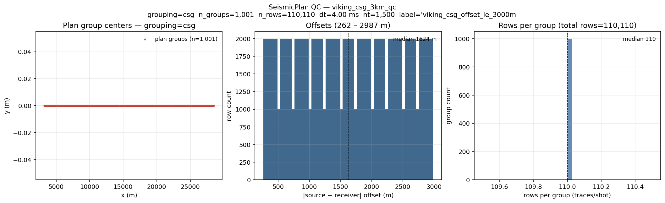
The regular white gaps in the offset histogram are not missing data: the group interval is 25 m, so offsets only ever take multiples of 25 m and some histogram bins have nothing that can land in them.
Inspect programmatically¶
python -c "from sweep_io.seismic_plan import SeismicPlan; \
           p=SeismicPlan.load('$VIKING_HOME/run/viking_csg_plan.npz'); \
           print(p.grouping, p.n_groups, p.n_rows); print(p.build_meta)"
Real output on Viking (full CSG plan):
i.e. 1,001 CSG groups (shots) × 120 traces each = 120,120 rows.
Full Viking CSG ~8 MB; offset-capped variants smaller. The plan
carries all four things FWI needs — row_source_xyz,
row_receiver_xyz, row_file_id, row_trace_offset — so Steps 3-6
never touch the raw SEG-Y header again.
Step 3 — Source wavelet¶
The wavelet that the FWI / RTM YAMLs reference is produced by a two-stage chain:
3a. rank-1 robust direct-wave average
       (per-shot estimate × 1001 shots → polarity-aligned → robust mean)
              │   average_direct_wavelet.npz
              ▼
3b. SIREN LBFGS prefit + sweep wave-equation refinement
       (SIREN MLP fits 3a, then refines via Acoustic forward solve)
              │   estimated_wavelet.npz   ← feeds FWI / RTM
              ▼
Optional: FarField.dat ASCII → npz (for QC comparison) ; 4-step pipeline plot
All four sub-stages are native sweep-tasks subcommands now:
analyze-wavelet, estimate-wavelet, convert-farfield,
plot-wavelet-steps. Input is the CSG SeismicPlan you built in
Step 2; output estimated_wavelet.npz plugs directly into the
wavelet: block of every FWI / RTM YAML in Steps 5 / 6.
What goes in / what comes out¶
| Stage | Input | Output | Measured cost on Viking |
|---|---|---|---|
3a analyze-wavelet |
SeismicPlan + SEG-Y | average_direct_wavelet.npz |
CPU, ~15 s (1001 shots, 8 threads) |
3b estimate-wavelet |
SeismicPlan + SEG-Y + 3a's npz | estimated_wavelet.npz |
1 GPU, ~15-30 min (1001-shot V100 reference) |
3c convert-farfield |
FarField.dat (ASCII) |
farfield_wavelet.npz |
CPU, ~1 s |
3d plot-wavelet-steps |
the 3a/3b/3c npz files | 4-panel comparison PNG | CPU, ~3 s |
3a — rank-1 robust direct-wave average¶
For each shot in [1..1001] the algorithm:
- picks the 4 nearest-offset receivers from the plan (offset is
|gx - sx|per row); - reads those four traces from SEG-Y via the plan's row-byte-offsets;
- computes predicted direct-arrival times
τ = |offset| / 1500 m/s; - runs rank-1 alternation in a
(-0.05 s, +0.30 s)window around each predicted arrival: alternately solve for one shared wavelet and per-trace amplitudes, ~25 iterations, until a single common wavelet shape explains all four traces in a least-squares sense; - records a residual-RMS-ratio per shot (residual ÷ observed within the direct window).
After all 1001 per-shot wavelets are estimated:
- drop shots with
residual_ratio > 0.5(noise / bad picks); - polarity-align the survivors against a preliminary median;
- drop shots whose shape correlation to the preliminary mean < 0.95;
- average the surviving wavelets; produce a causal version
(zero-pad the leading negative-time samples, peak at
t = 0).
Canonical Viking parameters (used in the reference run)¶
direct_batch:
  shot_start: 1
  shot_stop:  1001
  shot_stride: 1
  nearest_receivers: 4
  water_velocity_m_s: 1500
  rel_t_min_s: -0.05
  rel_t_max_s: 0.30
  iterations: 25
  min_residual_ratio: 0.5
  min_shape_corr_to_average: 0.95
Command¶
The YAML's analyze_wavelet: block carries the canonical Viking
parameters shown just above. To override one knob (e.g. test on
fewer shots), pass it on the CLI — overrides win:
Full-CLI form (no YAML) for reference:
sweep-tasks analyze-wavelet \
    --plan        $VIKING_HOME/run/viking_csg_plan.npz \
    --out-dir     $VIKING_HOME/run/wavelet/direct_batch \
    --shot-start 1 --shot-stop 1001 --shot-stride 1 \
    --nearest-receivers 4 \
    --water-velocity-m-s 1500 \
    --rel-t-min-s -0.05 --rel-t-max-s 0.30 \
    --iterations 25 \
    --min-residual-ratio 0.5 --min-shape-corr-to-average 0.95
CPU-only, no GPU needed. Wall time on Viking 1001 shots: ~15 s (measured end-to-end on a login node, 8 CPU threads).
Outputs (analysis/, average/)¶
analysis/wavelet_overlay_mean_std.png— every shot in light gray, ±1σ ribbon in blue, the robust average in dark blue. (This is the Visual-tour thumbnail.)analysis/wavelet_spectra_mean_std.png— amplitude spectrum of the same overlay.analysis/wavelet_residual_after_average.png— per-sample residual RMS after subtracting the average; sanity check that the rank-1 average actually explains each shot.analysis/wavelet_stats.csv— per-shot residual / shape-corr / used-in-average flag.average/average_direct_wavelet.npz— the robust mean. This is the input to Step 3b.summary.json,command.txt.
Reference numbers (Viking 1001 shots, verified end-to-end with sweep-tasks analyze-wavelet)¶
| metric | value |
|---|---|
| Shots used in robust average | 984 / 1001 |
| Median per-shot residual-ratio | 8.2 % |
| Median shape-correlation to mean | 0.994 |
Console output for the full run (measured end-to-end):
[analyze-wavelet] plan=/…/viking_csg_plan.npz
[analyze-wavelet] output_dir=/…/wavelet/direct_batch
  ...estimated 25 per-shot wavelets so far
  ...estimated 50 per-shot wavelets so far
  ...
  ...estimated 1000 per-shot wavelets so far
per-shot wavelet stack: (1001, 88)
[analyze-wavelet] average_wavelet_npz: …/average/average_direct_wavelet.npz
[analyze-wavelet] summary_json:        …/summary.json

real    0m14.665s
The wavelet shows the expected airgun signature — main pulse at ~0.05 s, bubble pulse at ~0.18 s.
3b — SIREN LBFGS prefit + sweep wave-equation refinement¶
3a gives a good average shape from the direct arrival only — it ignores reverberation off the sea surface and the deeper section. 3b refines this in two sub-steps so the wavelet matches the full recorded waveform in the FWI band:
   average_direct_wavelet.npz (rank-1; from 3a)
                  │  resample to SIREN time grid
                  ▼
   initial_wavelet_target.npz  ← LBFGS target
                  │  SIREN MLP: coords (-1..1) → wavelet samples
                  │  LBFGS minimise MSE(SIREN(t), target),  10 iter
                  ▼
   prefit_siren_wavelet.npz    ← prefit, matches target to ~1e-9
                  │  sweep Acoustic forward solve (4-shot batch)
                  │  filter obs + syn to 3-30 Hz
                  │  Adam on SIREN params, loss = trace_cosine + 0.05·MSE_prior
                  │  100 epochs (decreases ~9.3e-2 → ~8.1e-3 in 30 epochs)
                  ▼
   estimated_wavelet.npz       ← FEEDS FWI / RTM as wavelet.path
Two design choices worth knowing about:
- Why SIREN? A SIREN MLP regularises the wavelet to a smooth parameterisation that can still capture the bubble pulse without fitting noise. Direct sample-space inversion overfits in our experience.
- Why a prior? The wave-equation loss alone has a near-flat
direction (an overall time shift in the wavelet trades for a static
in the velocity model). The
prior_weight: 0.05term anchors the refined SIREN to the rank-1 average across the full band, killing that null space without over-constraining the bubble.
Canonical Viking parameters¶
wavelet_inversion:
  shot_start: 1
  shot_stop:  1001
  nearest_receivers: 4              # same selection as 3a, larger N is OK
  tmax_s: 6.0
  velocity_m_s: 1500                # background for the 1-D forward grid
  dx_m: 12.5   dz_m: 12.5
  x_padding_m: 500  z_padding_m: 500  model_depth_m: 360
  filter_lowcut_hz: 3.0
  filter_highcut_hz: 30.0
  filter_order: 4
  backend: cuda
  mode: siren
  epochs: 100
  lr: 1.0e-3
  loss_type: trace_cosine
  prefit_steps: 10
  prefit_lr: 1.0e-3
  initial_wavelet_prior_weight: 0.05
  inr_hidden_features: 64
  inr_hidden_layers: 3
  inr_first_omega0: 30.0
  inr_hidden_omega0: 30.0
Command¶
The YAML's estimate_wavelet: block carries all 20+ parameters
listed above. CLI flags still work for overrides — useful when
sweeping one hyperparameter:
Single GPU. Wall time on one V100: ~15-30 min. Use --backend eager
for a slow but GPU-architecture-independent fallback (CPU-only is also
viable for tiny --shot-stop values).
Expected outcome (production reference numbers)¶
For the full 1001-shot / 100-epoch / CUDA reference run:
trace-cosine loss falls from ~0.10 to ~0.012, and the final
wavelet correlates 0.90 with the 3a rank-1 average at zero lag.
The output PNGs (estimated_wavelet.png, wiggle_obs_syn_comparison.png,
spectrum_obs_syn_comparison.png) will be added to the Visual tour
once we capture a clean V100 reference run with the sweep-tasks
native CLI (the existing reference is from the legacy
fwi_workflow-dev pipeline; numbers are identical because the
algorithm is bit-exact, but the figure provenance differs).
Outputs (siren_pipeline/)¶
initial_wavelet_target.npz— rank-1 average resampled to SIREN time grid.prefit_siren_wavelet.npz— SIREN after LBFGS prefit (MSE → ~1e-9).estimated_wavelet.npz— final wavelet after the wave-equation main loop. This is what Step 5 / 6 YAMLs point at viawavelet.path.loss.csv,loss_curve.pngwiggle_obs_syn_comparison.png,spectrum_obs_syn_comparison.png— the 4-shot diagnostic batch used as the inversion target.final_filtered_records.npz,metadata.json,command.txt.
Reference numbers (Viking)¶
- Prefit MSE
1.6e-1 → 4.5e-10in 10 LBFGS iterations. - Wave-equation trace-cosine loss
9.3e-2 → 8.1e-3in 30 epochs, plateaus.
3c — Optional: convert FarField.dat for QC comparison¶
The SEG dataset includes the manufacturer-measured far-field
signature in FarField.dat (ASCII, one sample per line, dt = 4 ms).
You don't need it for FWI — the data-driven 3b output already feeds
everything — but it's a useful sanity check that the estimated wavelet
isn't wildly off:
(Or all-CLI: sweep-tasks convert-farfield --input $VIKING_HOME/raw/FarField.dat --out $VIKING_HOME/run/wavelet/farfield/farfield_wavelet.npz --dt-s 0.004.)
Writes farfield_wavelet.npz + .json metadata + .png QC plot
(time + spectrum; see Visual tour above). CPU-only, runs in ~1 s.
The PNG's top panel is the raw 4-ms-sampled signature (gray) and
the post-processed version (black; default identical because no
taper / zeroing was requested); the bottom panel is the
corresponding amplitude spectrum.
3d — Optional: 4-step pipeline plot¶
sweep-tasks plot-wavelet-steps --config $VIKING_HOME/viking.yaml
# → <pipeline-dir>/wavelet_pipeline_steps.png         (4-row stack)
# → <pipeline-dir>/wavelet_pipeline_steps_overlay.png (1-row overlay)
Renders a 4-panel time + frequency comparison: rank-1 average →
SIREN prefit → raw wave-equation output → post-processed final
wavelet. Reads three npz files under <pipeline-dir>:
initial_wavelet_target.npz, prefit_siren_wavelet.npz, and
estimated_wavelet.npz.
What it produces¶
Console output (~3 s wall):
[plot-wavelet-steps] stack   -> …/wavelet_pipeline_steps.png
[plot-wavelet-steps] overlay -> …/wavelet_pipeline_steps_overlay.png
- 1-row overlay (
wavelet_pipeline_steps_overlay.png) — all four pipeline outputs (rank-1 target → SIREN prefit → raw wave-equation output → post-processed final) superimposed in time and frequency so you can spot where each step actually changed the wavelet. - 4-row stack (
wavelet_pipeline_steps.png) — one row per pipeline step at the same y-axis range, useful for measuring small amplitude shifts step-by-step.
Both PNGs will be added to the Visual tour once a clean production
3b reference is captured with sweep-tasks estimate-wavelet.
Where the wavelet is (and is not) consumed¶
Step 5's frequency-selection inversion consumes NO wavelet at all — its misfit is invariant to the source spectrum, which is a large part of why it is the default path below. The wavelet from this step remains what you QC the data with, and what any conventional (non-encoded) FWI or the Step 6 RTM references via:
Edit the path: to point at wherever 3b wrote it on your machine —
$VIKING_HOME/run/wavelet/siren_pipeline/ if you followed the
examples above.
Step 4 — Initial velocity model (built in memory)¶
No tool, no legacy bridge, no file on disk: a marine FWI cold start is a water
layer over a 1-D gradient, and init_model.linear_gradient builds exactly that
inside the task YAML from four numbers:
init_model:
  name: vp
  shape: [320, 2285]          # 4.0 km x 28.56 km at dh = 12.5 m
  linear_gradient:
    vmin: 1996.0              # first sediment velocity
    vmax: 4416.0              # bottom of the model
    water_rows: 28            # 350 m of water, constant along the line
    water_vp: 1485.6          # measured from the direct arrival (Step 3a), not 1500
The top water_rows rows are stamped to exactly water_vp — which is also what
reparam.mask_water_layer keys on to pin the water column — and the ramp spans
the rows below the water, so the gradient's range is not eaten by it. No
lateral structure at all: nothing about the answer is smuggled into the start.
(A bathymetry-aware builder remains on the roadmap; the flat 28 rows are within
1-3 cells of the real seabed here, measured 343-372 m from the seabed
reflection.)
Step 5 — FWI with frequency-selection source encoding¶
The default inversion path for this example, and the reason it needs neither Step 3's wavelet nor any amplitude calibration:
- No wavelet enters the inversion. Every node in the active pool radiates
its own comb frequency continuously, and the misfit is per-node
complex-cosine coherence
J = 1 - |<u,d>| / (|u| |d|)on a steady-window DFT — invariant to any per-node complex scale, so the airgun spectrum, the excitation delay and the sensor coupling all cancel. - One forward per iteration for the whole pool, instead of one per shot:
| wavefield steps / iteration | 8 bands x 30 iter | measured | |
|---|---|---|---|
| conventional (96-168 shots x 6000 steps) | 576,000 | 190 M | ~4.5 h |
| frequency selection (one encoded pool) | 52,500 | 8.9 M | 10 min |
The encoded forward is ~9x longer than a single shot (ring-up + analysis window), so below ~9 shots conventional wins. Viking has 1001.
5a — Extract the observed coefficients¶
The obs side is a DTFT of gathers that already exist — no solver involved,
~20 s per band. A plan's groups become the nodes: CSG makes the 1001 shots
the nodes (their 120 receivers each are the traces), CRG
(--grouping crg --receiver-quantize-m 25) makes the 1131 receiver cells the
nodes. Either works — nodes carry their own receiver masks, so a moving
streamer spread is as valid as a fixed OBN patch, and on this line the two
give the same answer (51 % shallow two-init convergence either way).
mkdir -p $VIKING_HOME/run/shards
sweep-tasks extract-coeff --plan $VIKING_HOME/run/viking_csg_plan.npz \
    --dh-m 12.5 --dt 0.001 --min-fold 1 --node-stride 1 \
    --n-p 32000 --k-lo 96 --k-hi 192 \
    -o $VIKING_HOME/run/shards/coeff_3_6hz.npz
--dt is the solver dt — it defines the comb, f = k/(n_p*dt). The plan's
own 4 ms record dt is read from the plan and handled; the two are allowed to
differ. Repeat for the eight bands of the ladder:
| band | --n-p |
window | --k-lo |
--k-hi |
bins | nodes/iter | pools |
|---|---|---|---|---|---|---|---|
| 3-6 Hz | 32000 | 32 s | 96 | 192 | 97 | 96 | 11 |
| 3-8 | 20000 | 20 s | 60 | 160 | 101 | 96 | 10 |
| 3-10 | 18000 | 18 s | 54 | 180 | 127 | 120 | 8 |
| 3-12 | 14000 | 14 s | 42 | 168 | 127 | 120 | 8 |
| 3-14 | 14000 | 14 s | 42 | 196 | 155 | 144 | 7 |
| 3-16 | 12000 | 12 s | 36 | 192 | 157 | 144 | 7 |
| 3-18 | 12000 | 12 s | 36 | 216 | 181 | 168 | 6 |
| 2-20 | 10000 | 10 s | 20 | 200 | 181 | 168 | 6 |
How those numbers are derived — bins are the currency:
Pick the per-band pool size first (the batch size — 96-168 here, following the
survey's conventional-FWI schedule), then n_p >= pool / bandwidth / dt. The
window shortens as the ladder climbs, because a wider band reaches the same
bin count in less time: the lowest band is the expensive one. n_p does NOT
need to fit the 6 s record — the obs DTFT integrates whatever the record has;
n_p sizes the synthetic steady window whose exact DFT bins the encoded
sources must occupy. Each shard holds all 120,120 traces regardless of the
pool size — pools exist because 1001 nodes cannot each take an exclusive
frequency out of 97 bins, and random_batch redraws the subset every
iteration, exactly like shot mini-batching.
5b — Run it¶
cp ${SWEEP_TASKS}/examples/field/viking/viking_freqsel_8band.yaml \
   $VIKING_HOME/run/viking_freqsel.yaml
sweep-tasks run $VIKING_HOME/run/viking_freqsel.yaml
10 minutes on one RTX 6000 Ada for 8 bands x 30 iterations, peak 6.1 GB. Two parameters in that YAML are worth understanding before editing anything:
steady_samples: 20000— the continuous sources must ring up before the analysis window opens: model width / slowest velocity = 28.6 km / 1485.6 m/s = 19.2 s. The schema default (2500) leaves a transient in the window here.abcn: 50— the PML is sized by the LOWEST rung (2 Hz -> 743 m = 59 cells), because a continuous-wave field in a leaky box builds standing waves that do not cancel between a transient obs and a steady-state syn.
Repeat every key in every stage's
frequency:block. A stage block replaces the global one wholesale — it is not merged — so an omitted key silently reverts to the schema default (random_batch-> None turns random node batching back into deterministic rotation;steady_samples-> 2500 truncates the ring-up). The runner prints a warning naming each dropped key.
What "good" looks like¶
[freqsel] stage 0: 1001 nodes, 120120 items, 1131 union cells, 11 pools, ...
[freqsel][rank0] stage 0 steady-state two-window check: median rel diff = 1.7e-05
- two-window check
<= 1e-2(measured 1.6e-5..3.3e-5 across the ladder) — the runner extracts the coefficients twice,slack_samplesapart; if this fails, raisesteady_samples. - items = the survey's trace count (120,120): every (node, trace) pair is
in the misfit.
union cellsis the deduplicated receiver table — 120,120 pairs need only 1131 recording positions, with no loss of data. - water column pinned exactly:
max |vp[:28] - 1485.6| = 0. - per-band
mean(1-GCN)falls within every stage — reference run0.569 -> 0.467on the first band,0.322 -> 0.298on the last.
How far down to trust it¶
Run the same YAML from two different starting models and compare: where the data constrains the answer the results converge, where it does not each keeps its own start. Against the survey's own initial model (373 m/s RMSE from the linear start):
| depth | difference between the two results | convergence |
|---|---|---|
| 350-1000 m | 104 m/s | 51 % |
| 1000-2000 m | 449 | 3 % |
| 2000-3000 m | 461 | -1 % |
| 3000-4000 m | 344 | -6 % |
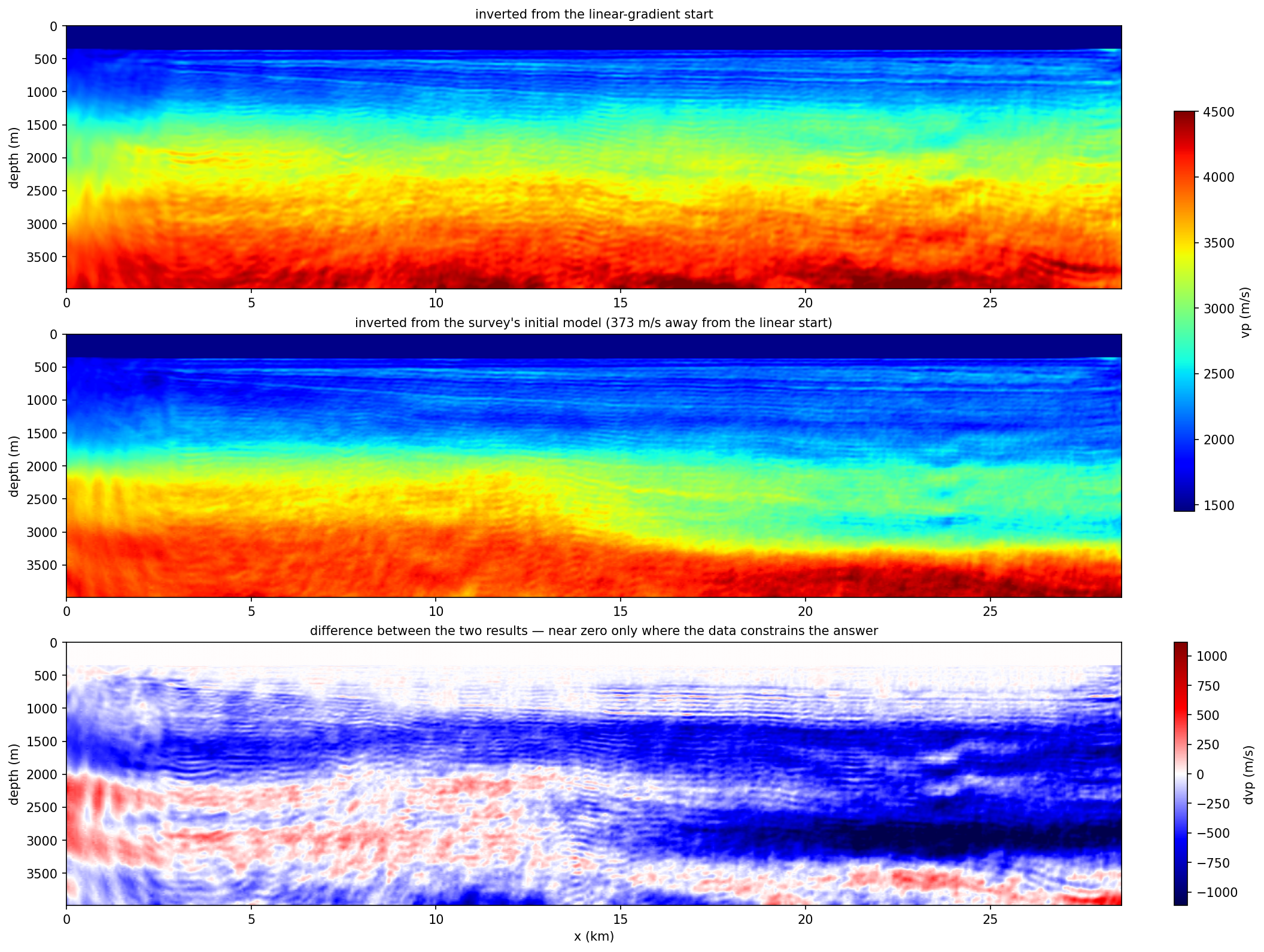
Only the top ~650 m of section is genuinely resolved by this 3.2 km-offset streamer dataset; structure below ~1000 m is inherited from the start, not an inversion result. That boundary survived a different hash geometry and 67 % more iterations unchanged — it is an illumination limit, not a tuning problem.
Known gaps of the reference run, left as exercises: model_bounds was not
enabled (vp reaches 1254 m/s in spots, below water velocity — set
model_bounds: {vp: {min: 1450, max: 5500}}); the water mask is a flat 28
rows rather than the measured 343-372 m bathymetry
(reparam.seabed_depth_path); and 30 iterations/band demonstrates the
workflow rather than converging it.
Step 6 — RTM with sweep-tasks run¶
Post-FWI imaging on the inverted vp at 12.5 m / 1 ms, 3-25 Hz band, illumination-normalised stack. Generate the annotated RTM template:
(Or copy the in-repo Viking-specific example
${SWEEP_TASKS}/examples/field/viking/viking_rtm_legacy_match.yaml.)
Point its velocity_model.path at your Step 5 output:
velocity_model:
  name: vp
  path: $VIKING_HOME/run/freqsel/viking_freqsel_8band/inverted_vp.npy
geometry:
  kind: from_plan
  plan_path: $VIKING_HOME/run/viking_csg_3km.npz     # 3 km plan from Step 2
obs:
  plan:
    plan_path: $VIKING_HOME/run/viking_csg_3km.npz
output_dir: $VIKING_HOME/run/viking_rtm
Run it:
Wall time: ~45 min on one V100 (1001 shots × one forward + one backward each, illumination-normalised stack).
Outputs (under $VIKING_HOME/run/viking_rtm/<task_id>/output/):
rtm_image.npy                          fwi_gradient_image.npy
rtm_image_normalised.npy               fwi_gradient_image_normalised.npy
rtm_image_per_shot_normalised.npy      fwi_gradient_image_per_shot_normalised.npy
rtm_result.npz                         (grid metadata + summary stats)
Preview figure to follow once a clean RTM reference run on the sweep-tasks CLI is captured.
Step 7 — Depth-tapered z-axis low-cut (post-filter)¶
Standard fix for shallow drift in the RTM image. Two equivalent routes:
Route A — standalone CLI (iterate on filter params, no GPU)¶
sweep-tasks filter-image \
    $VIKING_HOME/run/viking_rtm/viking_rtm_v1/output/rtm_image_per_shot_normalised.npy \
    --wavelength-m 300 --depth-m 600 --taper-m 400
# → rtm_image_per_shot_normalised_shallow_zlowcut.npy          (cleaned)
# → rtm_image_per_shot_normalised_shallow_zlowcut_removed.npy  (subtracted drift)
# → rtm_image_per_shot_normalised_shallow_zlowcut_*.png        (QC panels)
--dz-m is auto-read from the sibling rtm_result.npz; for non-sweep
inputs, pass it explicitly.
Route B — bake into the RTM YAML¶
imaging:
  shots_per_batch: 1
  filter_lowcut_hz: 3.0
  filter_highcut_hz: 25.0
  filter_target: syn
  normalize_by_illumination: true
  save_per_shot: false
  post_filter:
    enabled: true
    wavelength_m: 300.0
    depth_m: 600.0
    taper_m: 400.0
    targets: all
    save_png: true
One sweep-tasks run viking_rtm.yaml produces raw + filtered products
together. Full knob surface in
docs/cli_workflow.md.
Reproducibility cheat sheet (single GPU, local)¶
# === one-time setup ========================================================
export VIKING_HOME=$HOME/viking
mkdir -p $VIKING_HOME/{raw,run}

# === Step 0: download (~750 MB) ============================================
cd $VIKING_HOME/raw
BASE=https://s3.amazonaws.com/open.source.geoscience/open_data/Mobil_Avo_Viking_Graben_Line_12
curl -fL -O ${BASE}/seismic.segy
curl -fL -O ${BASE}/FarField.dat        # capital F twice — Farfield.dat is HTTP 403

# === one-time config =======================================================
sweep-tasks init -o $VIKING_HOME/viking.yaml

# === Steps 1-3d ============================================================
sweep-tasks build-index        --config $VIKING_HOME/viking.yaml
sweep-tasks build-plan         --config $VIKING_HOME/viking.yaml
sweep-tasks analyze-wavelet    --config $VIKING_HOME/viking.yaml
sweep-tasks estimate-wavelet   --config $VIKING_HOME/viking.yaml
sweep-tasks convert-farfield   --config $VIKING_HOME/viking.yaml
sweep-tasks plot-wavelet-steps --config $VIKING_HOME/viking.yaml

# === Step 4: initial model — nothing to run ================================
# (built in memory by init_model.linear_gradient inside the Step 5 YAML)

# === Step 5: freqsel FWI on one GPU (8 bands, ~10 min) =====================
SWEEP_TASKS=$(python -c "import sweep_tasks, pathlib; print(pathlib.Path(sweep_tasks.__file__).parent.parent.parent)")
mkdir -p $VIKING_HOME/run/shards
while read lo hi n_p klo khi; do
  sweep-tasks extract-coeff --plan $VIKING_HOME/run/viking_csg_plan.npz \
      --dh-m 12.5 --dt 0.001 --n-p $n_p --k-lo $klo --k-hi $khi \
      -o $VIKING_HOME/run/shards/coeff_${lo}_${hi}hz.npz
done <<'BANDS'
3 6 32000 96 192
3 8 20000 60 160
3 10 18000 54 180
3 12 14000 42 168
3 14 14000 42 196
3 16 12000 36 192
3 18 12000 36 216
2 20 10000 20 200
BANDS
cp ${SWEEP_TASKS}/examples/field/viking/viking_freqsel_8band.yaml $VIKING_HOME/run/viking_freqsel.yaml
sweep-tasks run $VIKING_HOME/run/viking_freqsel.yaml
# (multi-GPU on the same box: append --nproc-per-node N)

# === Step 6: RTM ===========================================================
cp ${SWEEP_TASKS}/examples/field/viking/viking_rtm_legacy_match.yaml $VIKING_HOME/run/viking_rtm.yaml
# …edit velocity_model.path + plan_path, then:
sweep-tasks run $VIKING_HOME/run/viking_rtm.yaml

# === Step 7: post-filter ===================================================
sweep-tasks filter-image \
    $VIKING_HOME/run/viking_rtm/viking_rtm_v1/output/rtm_image_per_shot_normalised.npy \
    --wavelength-m 300 --depth-m 600 --taper-m 400
Running on a cluster (optional)¶
For SLURM / ibex-style clusters the repo ships matching sbatch
templates under sweep-tasks/examples/sbatch/. They reference a
small set of environment roots — SWEEP_USER_ROOT,
SWEEP_STACK_ROOT, SWEEP_REPOS_ROOT, SWEEP_RUNS_ROOT,
SWEEP_CONDA_ROOT, PROJECT_DATA_ROOT — that you set in your login
shell rc before sbatch-ing. A working KAUST / ibex layout:
export SWEEP_USER_ROOT=/ibex/user/${USER}
export SWEEP_STACK_ROOT=${SWEEP_USER_ROOT}/sweep-stack
export SWEEP_REPOS_ROOT=${SWEEP_USER_ROOT}/repo
export SWEEP_RUNS_ROOT=${SWEEP_USER_ROOT}/runs
export SWEEP_CONDA_ROOT=${SWEEP_USER_ROOT}/miniconda3
export PROJECT_DATA_ROOT=/ibex/project/<your-allocation>   # holds the raw SEG-Y
Then:
# 4× V100 production FWI (6 stages, ~1 h 16 min wall)
sbatch ${SWEEP_STACK_ROOT}/sweep-tasks/examples/sbatch/viking_6stage_30hz.sbatch
# 1× V100 RTM
sbatch ${SWEEP_STACK_ROOT}/sweep-tasks/examples/sbatch/viking_rtm.sbatch
If you don't have or need SLURM, just stay with the sweep-tasks run
commands from Step 5 / 6 — that's what the sbatch scripts call
inside the allocation anyway.
Roadmap¶
What's in sweep-tasks today (sufficient for the entire Viking
workflow, end to end):
| Step | Subcommand | Notes |
|---|---|---|
| 1 | sweep-tasks build-index |
scan SEG-Y → SEGYIndex npz |
| 2 | sweep-tasks build-plan |
SEGYIndex + filters → SeismicPlan npz |
| 3a | sweep-tasks analyze-wavelet |
rank-1 robust direct-wave average (CPU) |
| 3b | sweep-tasks estimate-wavelet |
SIREN LBFGS prefit + sweep wave-equation refinement (1 GPU) |
| 3c | sweep-tasks convert-farfield |
ASCII FarField → npz adapter (CPU) |
| 3d | sweep-tasks plot-wavelet-steps |
4-panel pipeline QC plot (CPU) |
| 4 | init_model.linear_gradient |
in-memory water-layer + 1-D gradient (no tool needed) |
| 5a | sweep-tasks extract-coeff --plan |
field gathers → freqsel coefficient shards (CPU) |
| 5/6 | sweep-tasks run |
YAML-driven FWI (freqsel or conventional) / RTM |
| 7 | sweep-tasks filter-image |
depth-tapered z-low-cut on RTM images |
No legacy bridge remains: Step 4 is four numbers in the task YAML and
Step 5's misfit needs no wavelet, so sweep-tasks is self-contained
for Viking. Remaining nice-to-haves:
| Item | Notes |
|---|---|
| bathymetry-aware water mask | flat water_rows is 1-3 cells off the real seabed here; reparam.seabed_depth_path exists, a picker CLI does not |
| truncated freqsel backward | the adjoint source lives only in the probe window — backward could stop ~40-67 % early and the boundary store shrink to the tail; design noted, unimplemented |
CSG-index / SeismicPlan field mapping (for reference)¶
The wavelet port replaced the legacy csg_index_v2 npz reader with
sweep_io.SeismicPlan + PlanReader. If you're reading the legacy
scripts and trying to map field names:
Legacy csg_index_v2 field |
SeismicPlan equivalent |
|---|---|
shot_ids[i], shot_start[i], shot_count[i] |
plan.group_id[i], plan.group_offsets[i], plan.group_row_count(i) |
source_x_2d[row], receiver_x_2d[row] |
plan.row_source_xyz[row, 0], plan.row_receiver_xyz[row, 0] |
source_depth_m[row], receiver_depth_m[row] |
plan.row_source_xyz[row, 2], plan.row_receiver_xyz[row, 2] |
trace_offset[row] |
plan.row_trace_offset[row] |
offset[row] (signed) |
computed: sign(rx - sx) * hypot(rx - sx, ry - sy) |
read_traces_by_offset(segy_path, trace_offsets) |
PlanReader(plan).read_rows(row_idx) |
See also¶
docs/cli_workflow.md— generic build-index / build-plan / run reference (covers all datasets).examples/field/viking/*.yaml— every Viking task YAML, including the 6-stage and 8-stage FWI ladders and the legacy-matching RTM.examples/sbatch/viking_*.sbatch— matching ibex sbatch templates (cluster users only).fwi_workflow-dev/docs/datasets/viking/README.md— legacy reference (number-for-number equivalent through Step 6).