Anisotropic and elastic

Every other example pins equation: Acoustic or Acoustic3D — two of the 39 equations sweep-solver 0.3.5 registers, and two of only three that take vp alone. These two show the pattern for all the rest:

• models: must list every model the equation declares, by name, and the names are not guessable. Ask 15 rather than assume: AcousticVTI wants [vp, epsilon, delta], Elastic wants [vp, vs, rho], ElasticTTI wants eight. A missing or misspelt name is an error at setup, not a silent default.
• source_type / receiver_type are per-equation too. The acoustic h1 (pressure) still applies to VTI because it is pseudo-acoustic, but the velocity-stress elastic equation has no h1 at all. Get it wrong and the runner fails at setup with the full list of valid values.

Both build their models in memory, need no dataset, and run on impl: eager.

16 — VTI anisotropy

sweep-tasks run examples/synthetic/16_forward_anisotropic.yaml

A wavefront whose velocity depends on the direction it travels — which no isotropic example can show. Thomsen's parameters are defined so that zero means isotropy, so re-running with epsilon and delta both 0 is a clean control:

sweep-tasks run examples/synthetic/16_forward_anisotropic.yaml \
    --override task_id=aniso_iso \
    --override 'models=[{"name":"vp","constant":2500.0,"shape":[200,360]},
                        {"name":"epsilon","constant":0.0,"shape":[200,360]},
                        {"name":"delta","constant":0.0,"shape":[200,360]}]'

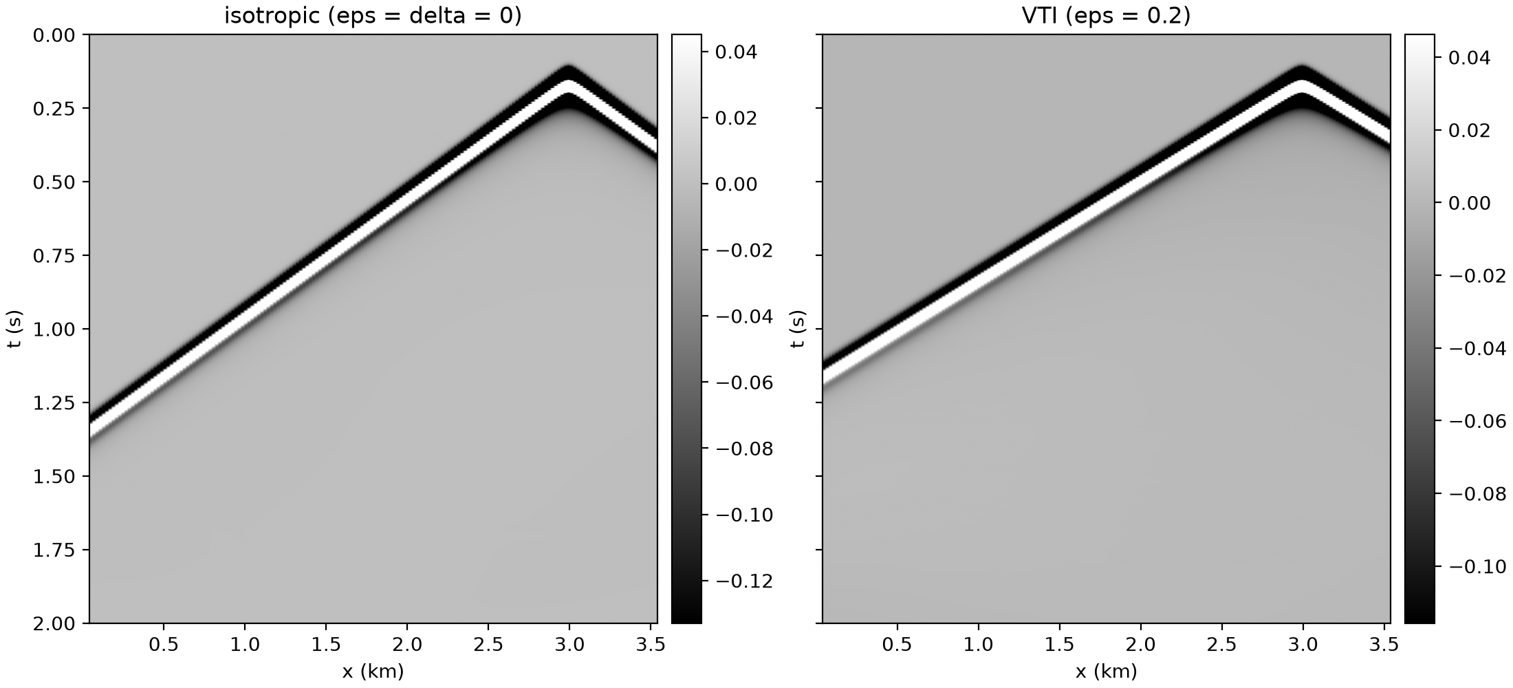
Same vp, same geometry: the VTI first break arrives earlier, and the gap grows with offset. Measured on the far-offset trace (1740 m) of shot 2:

	first break
isotropic, ε = δ = 0	787 ms
VTI, ε = 0.2	680 ms — ratio 1.157

The horizontal P velocity is vp·sqrt(1 + 2ε) = 1.183 vp, so 1.157 is the right answer rather than a near miss: at 1740 m with the source at 40 m and the receivers at 80 m the ray is not yet horizontal, so the measured speed-up must come in below the asymptote. delta controls the near-vertical curvature (the NMO velocity vp·sqrt(1 + 2δ)) rather than the horizontal asymptote.

Reference (--override device=cpu, 8 threads): 37.6 s, record (3, 2000, 176, 1).

17 — elastic: P and S in one record

sweep-tasks run examples/synthetic/17_forward_elastic.yaml

An explosive source in the elastic equation is equal normal stresses, source_type: [sxx, szz], and the natural receivers are the two particle-velocity components [vx, vz] — so the record's last axis is 2.

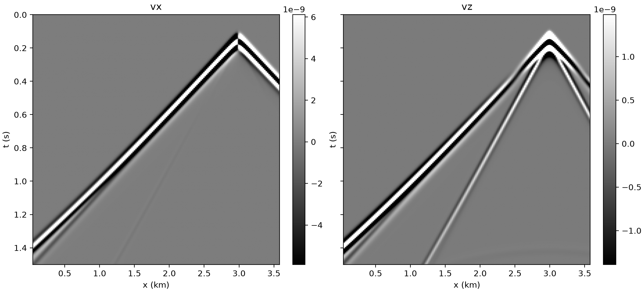
Two arrivals where the acoustic examples have one: the fast P and, steeper, the S wave. Measured on the far trace of shot 2 (vz), the two strongest arrivals land at 598.5 ms and 954.5 ms, a ratio of 1.59. The Poisson-solid vp/vs is 1.73, and 1.59 is right rather than a near miss: the models are gradients, so P and S turn at different depths and average different velocities on the way. Flatten the three gradients to constants and it goes to 1.73. At the first break vx carries 4–7× the amplitude of vz, which is what a near-horizontal direct P should do.

Set physics.free_surface: true and a third, slower, dispersive arrival appears — the Rayleigh wave — which does not exist in an acoustic model at all.

There is no pml_type: in the file, on purpose. Elastic is solved on a staggered grid, so its PML is the staggered cpmls; left unset, every equation gets the PML it ships, and naming another is refused.

Reference (--override device=cpu, 8 threads): 61.8 s, record (3, 3000, 178, 2).