iFWI — the model as a network

sweep-tasks run examples/synthetic/07_fwi_marmousi_inr.yaml

Same physics, same data, different unknowns. Instead of 382,441 velocity cells, the unknowns are the 251,728 weights of a coordinate network — a hash encoder feeding a SIREN — that is asked for vp(x, z) wherever the solver needs it. The optimiser trains the weights; the network's own smoothness is the regulariser. Everything about it lives in the reparam: block.

It starts from vp_smooth, the same start as 02, and runs the four-stage ladder and batch size of 03 for the same 200 epochs. The network predicts a perturbation added to the start (direct_velocity: false), so it begins near zero and the run begins exactly where 02 does.

Reference (RTX 6000 Ada, seed 0), 4 × 50 epochs, 13.9 min:

	grid (02)	network (07)
RMSE vs true	270.6	267.3
perturbation r	0.700	0.687
free parameters	382,441 cells	251,728 weights

A wash on accuracy, which is the honest result. What the parametrisation buys is a model with fewer degrees of freedom than the grid it renders onto.

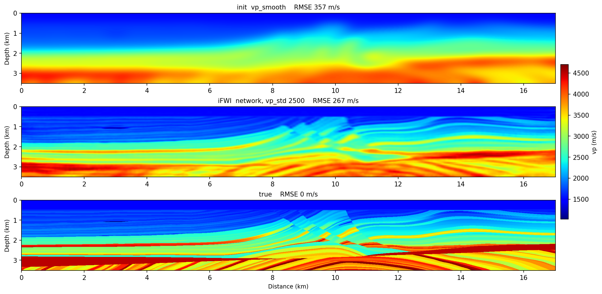
The one parameter that decides whether it works

reparam.vp_std. The network renders vp = init + raw * vp_std, and raw grows only as fast as lr × steps lets it — so vp_std is the effective step size in m/s, and lr is not. Size it to the perturbation the data needs, not to an intuition about small perturbations. Here the true update has rms 357 m/s and a range of ±1400:

vp_std	300	600	900	1500	2500	4000
RMSE	325.4	309.3	291.8	276.9	267.3	264.2
r	0.467	0.543	0.609	0.659	0.687	0.696

At 300 — the obvious first guess — the network saturates at ±180 m/s of update against the ±1400 the data is asking for, and the deep section barely moves (RMSE improves 1.2 % below 2.5 km). The curve flattens around 2500.